Continuous Monitoring of the Dowling Hall Footbridge
Research Team: Babak Moaveni (PI), Peter Moser (grad student), Iman Behmanesh (grad student), Xiang Li (grad student), Alyssa Kody (undergrad student)
Funding: NSF-BRIGE (1125624), Tufts FRAC
Duration: 5/2009 – 8/2014
Relevant publications to date:
Moser, P., and Moaveni, B. (2013). "Design and deployment of a continuous monitoring system for the Dowling Hall Footbridge." Experimental Techniques, 37(1), 15-26.
Kody, A., Li., X., and Moaveni, B. (2013). "Identification of physically simulated damage on a footbridge based on ambient vibration data." Proc. of the Structures Congress, ASCE, Pittsburgh, Pennsylvania, USA.
This page contains the following topics:
- Instrumentation (Phase I)
- Instrumentation (Phase II)
- Automated System Identification
- 17-Weeks of Ambient Vibration and Temperature Data
The Dowling Hall Footbridge on the Tufts campus provides a live laboratory for vibration-based structural health monitoring research and teaching.
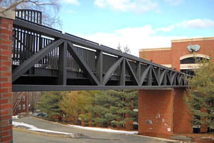
Figure 1. Dowling Hall Footbridge
Instrumentation (Phase I)
The first phase of installing a monitoring system on the Dowling Hall Footbridge was performed in the fall of 2009. Partial funding ($4,645) for this instrumentation was provided by the Tufts University Faculty Research Award Committee (FRAC). This system included an array of eight accelerometers and ten thermocouples, a rugged and remotely operable data acquisition system, and a reliable communication system. A set of data is recorded once an hour or when triggered by large vibrations. The system generates thousands of data records and development of programs automating the transfer, processing, and analysis of data was crucial to the success of the project. The monitoring system has been running continuously since January of 2010 and is still providing data. Figure 2 shows the location of accelerometers and thermocouples on the footbridge.
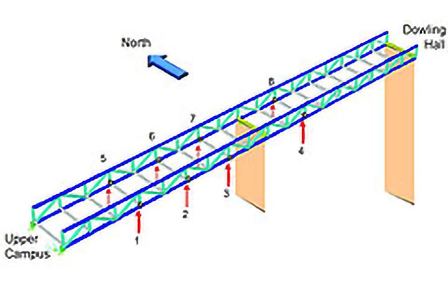
Figure 2a. Location of accelerometers
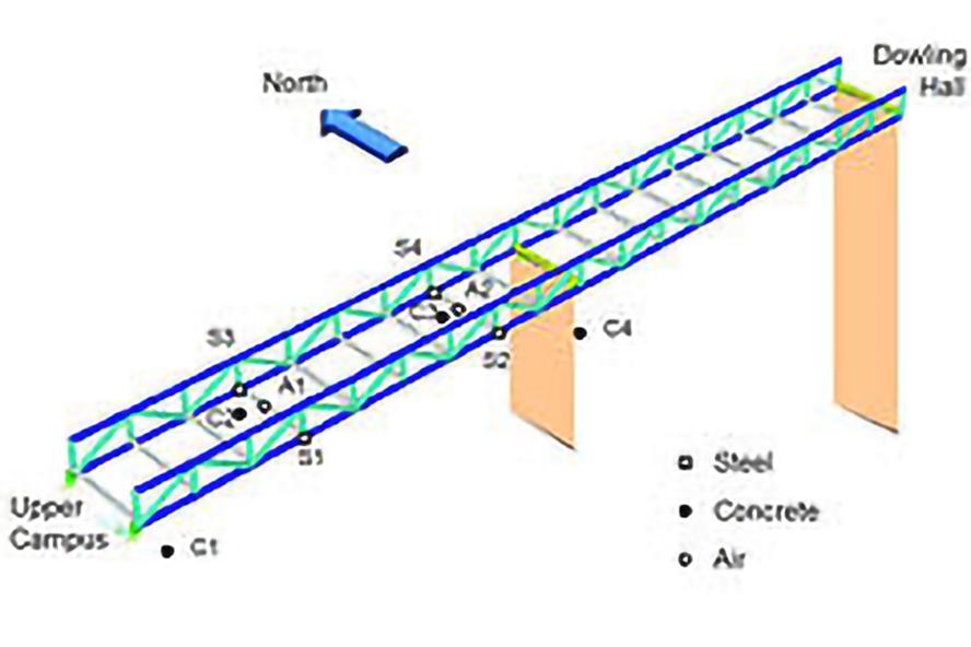
Figure 2b. thermocouples on the footbridge
Eight Piezoelectronics model 393B04 uniaxial accelerometers were permanently mounted to the underside of the bridge as shown in Figure 3. The current sensor network was found adequate for estimating the six lower vibration modes considered in this project. The monitoring system was designed to measure the air temperature, the steel frame temperature, the temperature of the heated concrete deck, and the temperature of the piers, all at several locations.
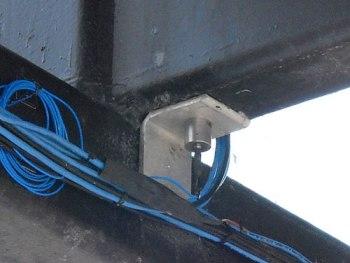
Figure 3. Installed accelerometer under the bridge
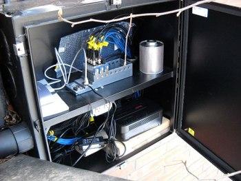
A National Instruments cRIO-9074 integrated chassis/controller is the core component of the data acquisition system. The ability to sample different sensors at different rates (acceleration vs. temperature) and direct on-chip scaling of raw data to account for channel sensitivities are two attractive features of the FPGA. Figure 4 shows the cRIO and three NI modules located inside a weatherproof enclosure next to the footbridge.
The monitoring program continuously samples the acceleration channels at a 2048 Hz sampling rate. Temperatures are recorded at a rate of one sample per second. A 5-minute data sample is recorded to the storage drive of the cRIO-9074 once each hour beginning at the top of the hour. The program also performs automatic triggering by continuously monitoring the one-second RMS value of each acceleration channel and will record a 5-minute sample if the values exceed 0.03 g. Sample recording can also be triggered manually.
Instrumentation (Phase II)
In the second phase of instrumentation of the DH Footbridge, four additional accelerometers and four strain gages were added on the bridge. The second phase of instrumentation was fully funded by the National Science Foundation (award no. 1125624) and was completed in April of 2012. The extra accelerometers were added on the piers (A11 and A12) and at the east side of the bridge (A9 and A10) as shown in Figure 5. Location of the four piezo-electric PCB 740B02 strain gages are also shown in Figure 5. The strain gages were attached to the prepared surface of the steel bottom cords under the bridge using epoxy (Figure 6a). After the installation of the strain gages, the locations where the paint was stripped were covered with black paint to prevent future rusting (Figure 6b).
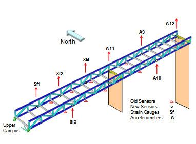
Figure 5. Layout of the added sensors during Phase II of instrumentation in April 2012
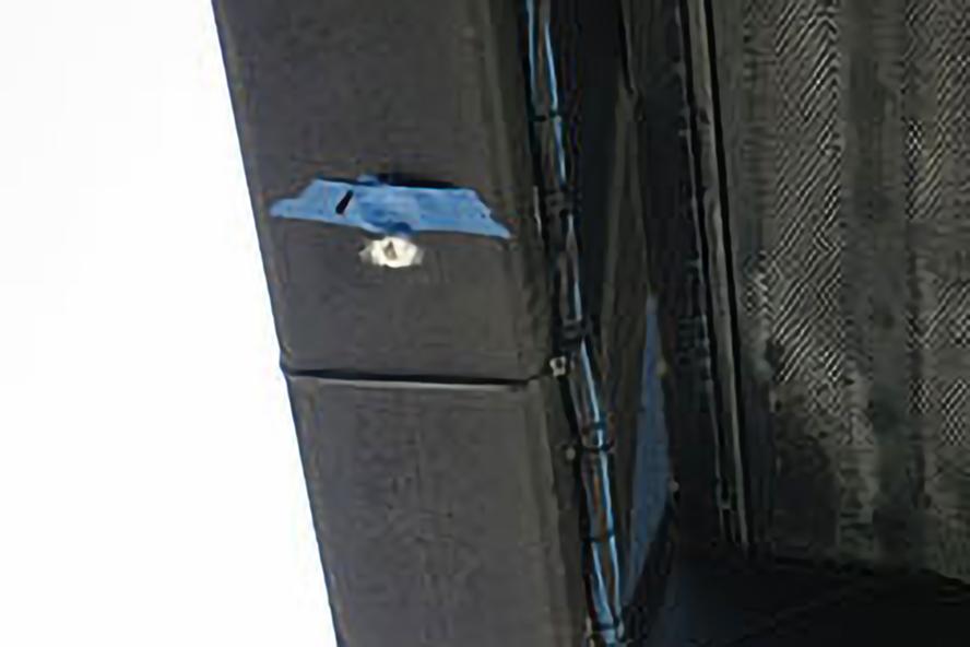
Figure 6a. Installed strain gage on prepared surface of the beam
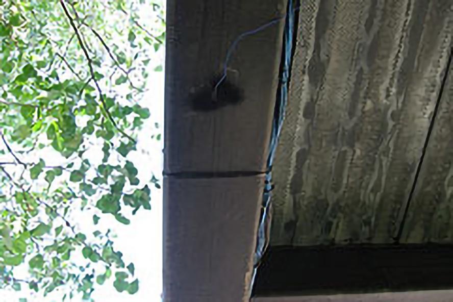
Figure 6b. Finished installation after painting the stripped paint spot
Automated System Identification
Once the data have been filtered and down-sampled, an automated stochastic subspace identification method is used for continuous modal analysis of the footbridge. Automatic modal analysis was completed for each of hourly measured records. A stabilization diagram is used to automatically select the physical modes of interest. Figure 7 shows the first six excited modes of the footbridge. Figure 8 shows a sample stabilization diagram.

Figure 7. Natural frequencies and mode shapes identified from a preliminary test on April 4, 2009
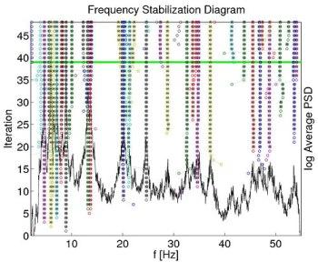
Figure 8. Sample stabilization diagram for data-driven SSI
The identified natural frequencies for a sixteen-week period beginning on January 5, 2010 and ending April 25, 2010 are shown in Figure 9. A clear pattern of daily variation in the natural frequencies can be observed. During this period, natural frequencies of the six identified modes varied by 4 to 8 percent while temperatures ranged from -14 to 39 °C. Because of this inherent variability in the natural frequencies, a model of the relationship between temperature and natural frequency must be developed before the dynamic characteristics of the bridge can be used for condition assessment.
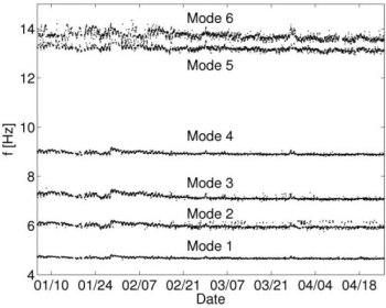
Figure 9. Variation of the natural frequencies of the first six modes during a 16-week period
17-Weeks of Ambient Vibration and Temperature Data
- Week 1: January 4-10, 2010 (.mat file)
- Week 2: January 11-17, 2010 (.mat file)
- Week 3: January 18-24, 2010 (.mat file)
- Week 4: January 25-31, 2010 (.mat file)
- Week 5: February 1-7, 2010 (.mat file)
- Week 6: February 8-14, 2010 (.mat file)
- Week 7: February 15-21, 2010 (.mat file)
- Week 8: February 22-28, 2010 (.mat file)
- Week 9: March 1-7, 2010 (.mat file)
- Week 10: March 8-14, 2010 (.mat file)
- Week 11: March 15-21, 2010 (.mat file)
- Week 12: March 22-28, 2010 (.mat file)
- Week 13: March 29-April 4, 2010 (.mat file)
- Week 14: April 5-11, 2010 (.mat file)
- Week 15: April 12-18, 2010 (.mat file)
- Week 16: April 19-25, 2010 (.mat file)
- Week 17: April 26-May 2, 2010 (.mat file)